01 · The four ways a correlation lies
Same picture, four different stories
When two measurements rise and fall together, the eye leaps to “one must cause the other”. But a correlation between A and B has at least four explanations, and only one of them is “A causes B”. Telling them apart is the whole discipline of causal inference; noticing that they exist is the whole of not being fooled.
A hidden third thing drives both
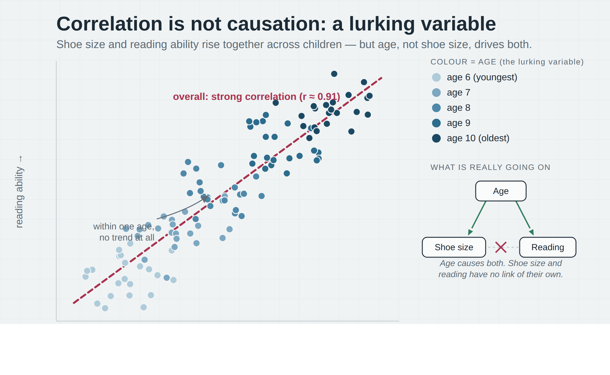
The most common culprit, and the one in the figure above. A confounder — age, wealth, the weather, the kind of person who does A — influences both variables at once, so they track each other with no direct link. Ice cream sales and drownings both follow the summer heat. See the interactive confounding explainer.
The arrow points the other way
Sometimes B causes A, not A causes B. People who take more medicine are sicker — but the medicine does not cause the illness; the illness causes the medicine. A bare correlation is silent on which end of the arrow is which.
Pure chance, given enough tries
Compare enough pairs of trending series and some will correlate for no reason at all — a country’s chocolate consumption and its Nobel prizes, or the divorce rate and margarine sales. Trends make it worse, and searching many pairs makes it certain. Watch it happen in the spurious correlation machine.
The way the data was gathered made the link
Filtering the data can create a correlation that is not there in the world — conditioning on a common effect (a collider) links its causes. Among hospital patients, or on a dating shortlist, two unrelated traits can appear to trade off. See Berkson’s paradox.
02 · The lurking variable
How the figure fakes a link
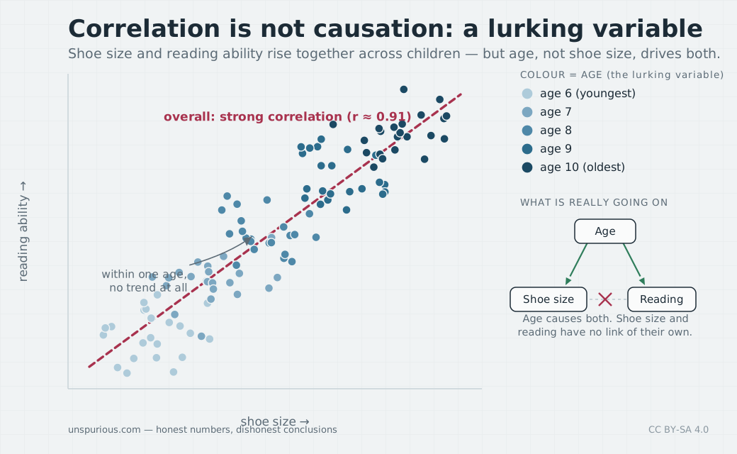
The scatter at the top is the textbook case, and it is worth reading slowly. Take a hundred schoolchildren and plot each one’s shoe size against their reading score, and you get a strikingly strong correlation — about 0.9, the kind of number a research paper would call a firm finding. Read literally, it says bigger feet come with better reading.
They do — but not because feet help you read. Colour each dot by the child’s age and the secret spills out: the youngest children sit low and to the left, the oldest high and to the right, and the whole diagonal band is just the march from young to old. Age is the lurking variable. It makes feet grow and reading improve, quite separately, so the two ride along together with no thread between them. The proof is in the colours: hold age fixed — look inside any single shade — and the trend vanishes into a shapeless cloud. On two children of the same age, the one with bigger feet is no more likely to read better.
This is confounding, and when the lurking variable is strong enough it can do worse than fake a link — it can reverse one, so a trend that holds in every subgroup points the opposite way once the groups are pooled. That extreme is Simpson’s paradox, and you can build one by hand.
03 · Breaking the tie
What it takes to earn the word “cause”
If a correlation can be four different things, how does anyone ever establish a cause? The gold standard is a randomised controlled experiment. Assign who gets the treatment by the flip of a coin and chance spreads every confounder — the ones you thought of, the ones you didn’t, and the ones nobody has named — evenly across the groups. If an effect then appears, the treatment is the only thing that systematically differs, so it earns the right to be called the cause. It is why the whole apparatus of clinical trials exists, and why “people who take vitamin X live longer” so often evaporates when someone finally randomises it.
When an experiment is impossible — you cannot randomise people to smoke, or to be poor — a cause can still be argued for, but only by hard, contestable work: measuring and adjusting for the confounders you can think of, checking that the supposed cause comes before the effect, looking for a dose-response pattern and a plausible mechanism, and asking whether any unmeasured lurking variable could be large enough to explain the whole thing away. Those are, in essence, the Bradford Hill considerations, and they are how the link between smoking and lung cancer was established without a single randomised human trial. The bar is high on purpose. A correlation opens the question of cause; it never closes it.
References & further reading
Sources
- Huff, D. (1954). How to Lie with Statistics. New York: W. W. Norton. — the classic popular treatment of statistical misuse, including spurious correlation.
- Pearl, J. & Mackenzie, D. (2018). The Book of Why: The New Science of Cause and Effect. New York: Basic Books. — confounders, colliders and the modern logic of causal inference.
- Fisher, R. A. (1935). The Design of Experiments. Edinburgh: Oliver & Boyd. — randomisation as the basis for causal inference.
- Hill, A. B. (1965). “The Environment and Disease: Association or Causation?” Proceedings of the Royal Society of Medicine, 58(5), 295–300. — the criteria for inferring causation from observational data.
- Simpson, E. H. (1951). “The Interpretation of Interaction in Contingency Tables.” Journal of the Royal Statistical Society, Series B, 13(2), 238–241.
- Messerli, F. H. (2012). “Chocolate Consumption, Cognitive Function, and Nobel Laureates.” New England Journal of Medicine, 367(16), 1562–1564. doi:10.1056/NEJMon1211064 — a tongue-in-cheek confounded correlation.
- Matthews, R. (2000). “Storks Deliver Babies (p = 0.008).” Teaching Statistics, 22(2), 36–38. — a memorable teaching example of a confounded correlation.